Why a Positive Test Result Doesn’t Always Mean You Have the Condition

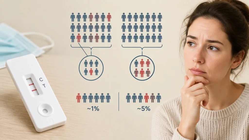
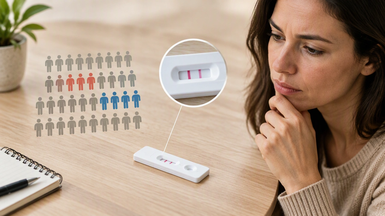
A positive medical test can feel like a final answer, but the result is only one part of the story. The same positive result can mean a high probability of disease in one setting and a low probability in another. The missing ingredient is the base rate: how common the condition is in the group being tested. This is a practical example of probability, and it shows why understanding false positives with conditional probability is essential.

Start with the question the result actually answers

A test result is evidence, not a diagnosis. The useful question is not simply, “What is the chance the test is positive?” It is the reverse question: “Given that the test is positive, what is the chance the condition is present?”

That reversal matters. The chance of seeing a positive result among people who have the condition is different from the chance of having the condition after seeing a positive result. Confusing these two directions is a classic probability error.

To reason clearly, define three quantities:

• Prevalence: the share of the tested population that has the condition.
• Sensitivity: the probability that the test is positive when the condition is present.
• Specificity: the probability that the test is negative when the condition is absent.

The false positive rate is one minus specificity: the probability that the test is positive when the condition is absent.

A concrete example with a rare condition

Suppose a screening program tests 10,000 people. Assume the condition has a prevalence of 1%, so 100 people have it and 9,900 do not.

Suppose the test has 95% sensitivity and 95% specificity. Among the 100 people with the condition, 95 test positive and 5 test negative. Among the 9,900 people without the condition, 495 test positive and 9,405 test negative.

Now collect the positive results: 95 true positives plus 495 false positives, giving 590 positive results in total. The proportion of positive results that correspond to the condition is 95 divided by 590, which is about 16.1%.

So, in this example, a positive result means there is roughly a 16% chance that the condition is present. The test performs well on each group separately, yet most positive results are false positives because the condition is rare and the unaffected group is large.

Why the base rate changes the answer

The key is the size of the two groups. With a 1% prevalence, there are many more people without the condition than with it. Even a modest false positive rate can therefore produce more false positives than true positives.

Change only the prevalence and the conclusion changes. If the same test is used in a high-risk group where prevalence is 20%, the calculation gives 190 true positives and 1,600 false positives among 1,000 affected and 4,000 unaffected people. The positive predictive value is 190 divided by 1,790, or about 10.6%.

Wait, that comparison uses different group sizes, so keep the total population constant to see the effect cleanly. Return to 10,000 people, but assume 20% prevalence: 2,000 have the condition and 8,000 do not. With the same sensitivity and specificity, true positives number 1,900 and false positives number 400. The positive predictive value is 1,900 divided by 2,300, or about 82.6%.

The test characteristics did not change. The base rate did, and that alone moved the interpretation from a minority chance to a strong likelihood.

The conditional probability view

Let D mean the condition is present and let T+ mean a positive test. The desired quantity is the conditional probability of D given T+, written P(D | T+).

Using the definition of conditional probability:

P(D | T+) = P(T+ | D) × P(D) / P(T+)

Here, P(T+ | D) is sensitivity, P(D) is prevalence, and P(T+) is the total probability of a positive result. The denominator includes both true positives and false positives:

P(T+) = P(T+ | D) × P(D) + P(T+ | not D) × P(not D)

For the 1% example, the numerator is 0.95 × 0.01 = 0.0095. The denominator is 0.0095 + 0.05 × 0.99 = 0.0095 + 0.0495 = 0.059. Dividing gives 0.0095 / 0.059 ≈ 0.161, matching the earlier count.

What this means for interpreting results

Several practical lessons follow from the arithmetic:

• Context matters: A positive result in a low-prevalence population carries less evidential weight than the same result in a high-prevalence population.
• Confirmatory testing helps: A second, independent test can reduce uncertainty because two false positives are less likely to occur together, though no test is perfect.
• Thresholds involve trade-offs: Making a test more sensitive can increase false positives unless specificity is also considered.
• Communication should include probabilities: Saying “positive” without explaining the chance of actually having the condition can mislead.

Screening decisions also depend on the consequences of missing a case versus following up on a false alarm. Those consequences are medical and ethical questions, but the underlying calculation is the same: combine the test’s conditional performance with the population’s base rate.

A habit of careful thinking

Base rates are easy to overlook because a positive result feels concrete and a prevalence figure feels abstract. Conditional probability restores the missing context. It asks not only how often a test produces a signal, but how likely the signal is to point to the truth in the population being examined.

The broader lesson applies beyond medicine: when a rare event is screened by an imperfect detector, false positives can dominate. The calm, disciplined response is to locate the base rate, state the test’s sensitivity and specificity, and calculate the reverse conditional probability before drawing a conclusion. That is how a positive result becomes interpretable rather than alarming.