How to Use Bayes’ Theorem to Update Probabilities

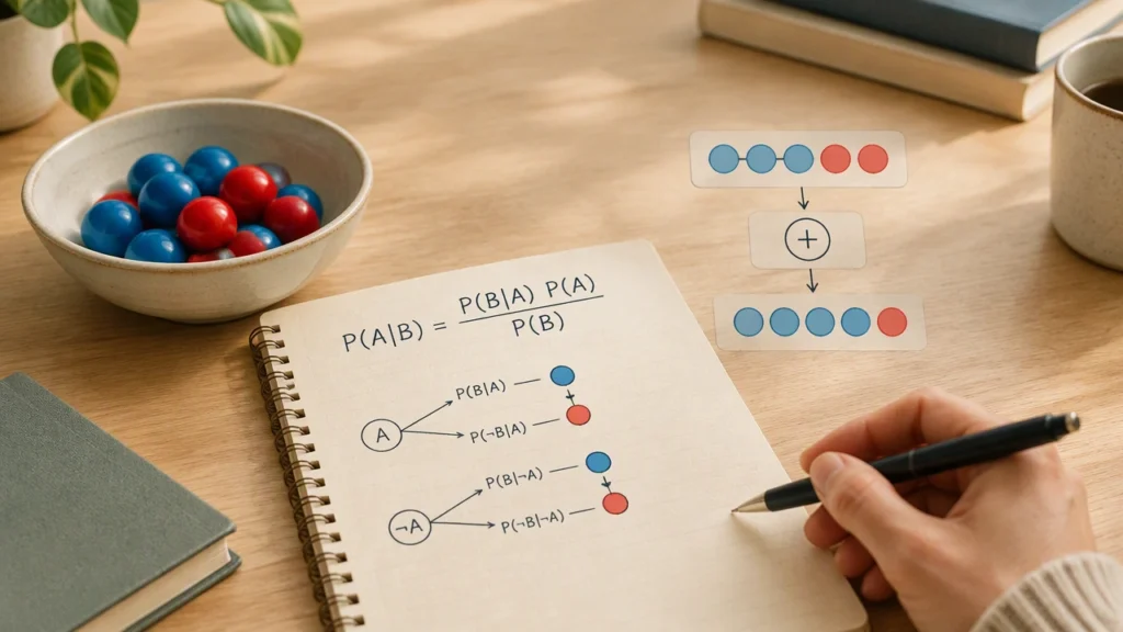
Probability gives us a language for uncertainty. It helps us describe what might happen, how likely different outcomes are, and how those likelihoods change when we learn something new. One of the most useful ideas in this field is learning how to use Bayes’ theorem to update probabilities in a disciplined way.

Bayes’ theorem is not a magic predictor. It is a rule for revising a belief in light of evidence. The approach is widely used in medicine, engineering, forecasting, machine learning, and everyday reasoning. This introduction explains the core idea, the formula, and a careful example without assuming prior training in advanced mathematics.

Start with conditional probability

Conditional probability is the probability of one event given that another event has occurred. If we write A and B for two events, the conditional probability of A given B is written P(A | B). The vertical bar means “given.”

For example, the chance that a randomly selected person has a certain symptom is different from the chance that they have the symptom after learning that they tested positive for a related condition. The second quantity is conditional because the new information changes the situation.

A useful starting point is the definition:

P(A | B) = P(A and B) / P(B)

This expression says that, once we know B happened, we only care about outcomes inside B. The probability of A and B is then divided by the total probability of B to rescale it. Rearranging this definition gives the multiplication rule:

P(A and B) = P(B | A) P(A)

Because the same joint probability can also be written as P(A | B) P(B), we can set the two forms equal and divide by P(B). That produces Bayes’ theorem.

Bayes’ theorem in plain language

The most common form of the theorem is:

P(H | E) = [P(E | H) P(H)] / P(E)

Here H is a hypothesis, such as “the machine is faulty,” and E is evidence, such as “the sensor reports an error.” The terms have names that make the logic easier to follow:

• P(H) is the prior probability: what we believed before seeing the evidence.
• P(E | H) is the likelihood: how probable the evidence is if the hypothesis is true.
• P(E) is the total probability of the evidence, under all relevant possibilities.
• P(H | E) is the posterior probability: the updated belief after seeing the evidence.

The theorem says that a strong prior can remain strong, and a weak prior can grow, but both are influenced by how well the evidence matches the hypothesis. Evidence that is much more likely when H is true than when H is false pushes the posterior upward. Evidence that is equally likely under both possibilities leaves the odds largely unchanged.

Calculating the denominator

The term P(E) can be found with the law of total probability. If H and its complement are the only possibilities, then:

P(E) = P(E | H) P(H) + P(E | not H) P(not H)

This step matters because it prevents an intuitive mistake: focusing only on how likely the evidence is when the hypothesis is true. The same evidence may also be fairly likely when the hypothesis is false. The denominator accounts for both paths.

In practice, it is often easier to compare odds rather than work with percentages directly. The odds form of Bayes’ theorem states:

posterior odds = prior odds x likelihood ratio

The likelihood ratio is P(E | H) divided by P(E | not H). It measures the diagnostic strength of the evidence. A ratio near 1 carries little information; a ratio much larger than 1 supports H strongly.

A worked example

Suppose a quality check examines a batch of sensors. Historically, 2% of sensors have a calibration fault, so the prior probability of a fault is P(F) = 0.02. A diagnostic test is used. If a sensor is faulty, the test flags it with probability 0.9. If it is not faulty, the test still flags it with probability 0.05, reflecting a false positive rate.

What is the probability that a flagged sensor is faulty? First calculate the total probability of a flag:

P(flag) = (0.9 x 0.02) + (0.05 x 0.98) = 0.018 + 0.049 = 0.067

Now apply Bayes’ theorem:

P(F | flag) = (0.9 x 0.02) / 0.067 = 0.018 / 0.067 = approximately 0.269

So the updated probability is about 26.9%. The flag raises the chance of a fault from 2% to roughly one in four. The result is higher than the prior, but it is not close to certainty. The low base rate of faults means that many flags come from the much larger group of non-faulty sensors.

Why the update is not the final answer

A posterior probability is a snapshot based on stated assumptions. If the prior is wrong, the likelihoods are miscalibrated, or the evidence is not independent, the result can be misleading. Real-world data may also change over time, so the posterior from one round can become the prior for the next.

It is equally important to avoid overconfidence. A single test result is not a verdict. Sequential updating is often more informative: observe evidence, revise the probability, then revise again as new evidence arrives. This is why Bayes’ theorem is useful for learning from repeated observations rather than making a one-time judgment.

Practical habits for clearer reasoning

• State the hypothesis precisely. “The device is faulty” is more useful than “something is wrong.”
• Separate prior from likelihood. Record what you assumed before seeing the evidence and how the evidence would behave under each possibility.
• Check the base rate. Rare events often remain uncommon even after a positive signal.
• Use sensitivity analysis. Recalculate with a few plausible priors or error rates to see how stable the conclusion is.
• Update over time. Treat each new observation as a chance to refine, not replace, your understanding.

Bayes’ theorem offers a clear way to update beliefs without ignoring what came before. By combining a prior, a likelihood, and the total probability of the evidence, it turns intuition into a transparent calculation. Used carefully, it helps us reason about uncertainty with patience, consistency, and respect for the limits of our information.